図8.1: stationaryDistribution
In this chapter, we will explain the sampling method. This time, we will focus on a sampling method called MCMC (Markov Chain Monte Carlo), which samples multiple appropriate values from a certain probability distribution.
The simplest method for sampling from a certain probability distribution is the rejection method, but sampling in a three-dimensional space has a large rejected area and cannot withstand actual operation. Therefore, the content of this chapter is that by using MCMC, sampling can be performed efficiently even in high dimensions.
As for the information about MCMC, on the one hand, systematic information such as books is for statisticians, and there is no guide to implementation for programmers, although it is redundant, and on the other hand, the information on the net has more than 10 lines of sample code. The reality is that there is no content that allows you to quickly and comprehensively understand the theory and implementation, as it is only described and there is no care for the theoretical background. I tried to make the concrete explanations in the following sections as such as possible.
The explanation of the probability that is the background of MCMC is enough to write one book if it is strictly speaking. This time, with the motto of explaining the minimum theoretical background that can be implemented with peace of mind, we aimed for an intuitive expression with moderate strictness of definition. I think that if you have used mathematics in the first year of university or even a little at work, you can read the program without difficulty.
In this chapter, the Unity project of Unity Graphics Programming https://github.com/IndieVisualLab/Assets/ProceduralModeling in UnityGraphicsProgramming is prepared as a sample program.
To understand the theory of MCMC, we first need to understand the basics of probability. However, there are few concepts to keep in mind in order to understand MCMC this time, only the following four. No likelihood or probability density function required!
Let's look at them in order.
When an event occurs at establishment P (X), this real number X is called a random variable. For example, when "the probability of getting a 5 on a dice is 1/6", "5" is a random variable and "1/6" is a probability. In general, the previous sentence can be rephrased as "the probability that an X on the dice will appear is P (X)".
By the way, if you write it a little like a definition, the random variable X is a mapping X that returns a real number X for the element ω (= one event that happened) selected from the sample space Ω (= all the events that can occur). You can write = X (ω).
I added a slightly confusing definition in the latter half of the random variable because it makes it easier to understand the stochastic process on the assumption that the random variable X is represented by the notation X = X (ω). The stochastic process is the one that can be expressed as X = X (ω, t) by adding the time condition to X. In other words, the stochastic process can be thought of as a kind of random variable with a time condition.
The probability distribution shows the correspondence between the random variable X and the probability P (X). It is often represented by a graph with probability P (X) on the vertical axis and X on the horizontal axis.
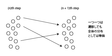
Each point is a distribution in which the overall distribution does not change even if it transitions. For a transition matrix π with a distribution P, P that satisfies πP = P is called a stationary distribution. This definition alone is confusing, but it is clear from the figure below.
図8.1: stationaryDistribution
Now, in this section, we will touch on the concepts that make up MCMC.
As mentioned at the beginning, MCMC is a method of sampling an appropriate value from a certain probability distribution, but more specifically, the Monte Carlo method under the condition that the given distribution is a steady distribution. (Monte Carlo) and Markov chain (Markov chain) sampling method. Below, we will explain the Monte Carlo method, Markov chain, and stationary distribution in that order.
The Monte Carlo method is a general term for numerical calculations and simulations that use pseudo-random numbers.
An example that is often used to introduce numerical calculations using the Monte Carlo method is the following calculation of pi.
float pi;
float trial = 10000;
float count = 0;

for(int i=0; i<trial; i++){
    float x = Random.value;
    float y = Random.value;
    if(x*x+y*y <= 1) count++;
}

pi = 4 * count / trial;
In short, the ratio of the number of trials in a fan-shaped circle in a 1 x 1 square to the total number of trials is the area ratio, so the pi can be calculated from that. As a simple example, this is also the Monte Carlo method.
A Markov chain is a stochastic process that satisfies Markov properties, in which states can be described discretely.
Markov property is the property that the probability distribution of the future state of a stochastic process depends only on the current state and not on the past state.
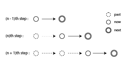
Figure 8.2: Markov Chain
As shown in the above figure, in the Markov chain, the future state depends only on the current state and does not directly affect the past state.
MCMC needs to use pseudo-random numbers to converge from an arbitrary distribution to a given stationary distribution. This is because if you do not converge to a given distribution, you will sample from a different distribution each time, and if you do not have a stationary distribution, you will not be able to sample well in a chain. In order for an arbitrary distribution to converge to a given distribution, the following two conditions must be met.
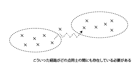
図8.3: Irreducibility
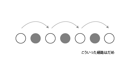
Figure 8.4: Aperiodicity
Any distribution that meets these two conditions can converge to a given stationary distribution. This is called the ergodic nature of the Markov process.
Now, it is difficult to check whether the given distribution satisfies the ergonomics mentioned earlier, so in many cases, we will strengthen the conditions and investigate within the range that satisfies the condition of "detailed balance". One of the Markov chain methods that achieves detailed balance is called the metropolis method.
The metropolis method samples by taking the following two steps.
The merit of the metropolis method is that even after the transition to the maximum value of the probability distribution is completed, if the value of r is small, the probability value transitions to the smaller one, so sampling proportional to the probability value can be performed around the maximum value.
By the way, the Metropolis method is a kind of Metropolis-Hastings method (MH method). The Metropolis method uses a symmetrical distribution for the proposed distribution, but the MH method does not.
Let's take a look at the actual code excerpt and see how to implement MCMC.
First, prepare a three-dimensional probability distribution. This is called the target distribution. This is the "target" distribution because it is the distribution you actually want to sample.
void Prepare()
{
    var sn = new SimplexNoiseGenerator();
    for (int x = 0; x < lEdge; x++)
        for (int y = 0; y < lEdge; y++)
            for (int z = 0; z < lEdge; z++)
            {
                var i = x + lEdge * y + lEdge * lEdge * z;
                var val = sn.noise(x, y, z);
                data[i] = new Vector4(x, y, z, val);
            }
}
This time, we adopted simplex noise as the target distribution.
Next, actually run MCMC.
public IEnumerable<Vector3> Sequence(int nInit, int limit, float th)
{
    Reset();

    for (var i = 0; i < nInit; i++)
        Next(th);

    for (var i = 0; i <limit; i ++)
    {
        yield return _curr;
        Next(th);
    }
}
public void Reset()
{
     for (var i = 0; _currDensity <= 0f && i < limitResetLoopCount; i++)
     {
             _curr = new Vector3(
               Scale.x * Random.value,
               Scale.y * Random.value,
               Scale.z * Random.value
               );
             _currDensity = Density(_curr);
     }
}
Run the process using a coroutine. Since MCMC starts processing from a completely different place when one Markov chain ends, it can be conceptually considered as parallel processing. This time, I use the Reset function to run another process after a series of processes. By doing this, you will be able to sample well even if there are many maxima of the probability distribution.
Since the first part of the transition is likely to be a point away from the target distribution, this section is burn-in without sampling. When the target distribution is sufficiently approached, sampling and transition set are performed a certain number of times, and when finished, another series of processing is started.
Finally, it is the process of determining the transition.
Since it is three-dimensional, the proposed distribution uses a trivariate standard normal distribution as follows.
public static Vector3 GenerateRandomPointStandard()
{
        var x = RandomGenerator.rand_gaussian(0f, 1f);
        var y = RandomGenerator.rand_gaussian(0f, 1f);
        var z = RandomGenerator.rand_gaussian(0f, 1f);
        return new Vector3(x, y, z);
}
public static float rand_gaussian(float mu, float sigma)
{
     float z = Mathf.Sqrt(-2.0f * Mathf.Log(Random.value))
              * Mathf.Sin(2.0f * Mathf.PI * Random.value);
     return mu + sigma * z;
}
In the Metropolis method, the distribution must be symmetrical, so the mean value is not set to anything other than 0, but if the variance is set to something other than 1, it is derived as follows using the Cholesky decomposition. I will.
public static Vector3 GenerateRandomPoint(Matrix4x4 sigma)
{
    var c00 = sigma.m00 / Mathf.Sqrt(sigma.m00);
    var c10 = sigma.m10 / Mathf.Sqrt(sigma.m00);
    var c20 = sigma.m21 / Mathf.Sqrt(sigma.m00);
    var c11 = Mathf.Sqrt (sigma.m11 - c10 * c10);
    var c21 = (sigma.m21 - c20 * c10) / c11;
    var c22 = Mathf.Sqrt(sigma.m22 - (c20 * c20 + c21 * c21));
    var r1 = RandomGenerator.rand_gaussian(0f, 1f);
    var r2 = RandomGenerator.rand_gaussian(0f, 1f);
    var r3 = RandomGenerator.rand_gaussian(0f, 1f);
    var x = c00 * r1;
    var y = c10 * r1 + c11 * r2;
    var z = c20 * r1 + c21 * r2 + c22 * r3;
    return new Vector3(x, y, z);
}
To determine the transition destination, take the ratio of the probabilities of the proposed distribution (one point above) next and the immediately preceding point_curr on the target distribution, and if it is larger than a uniform random number, it will transition, otherwise it will not transition. I will.
Since the process of finding the probability value corresponding to the coordinates of the transition destination is heavy (the amount of processing of O (n ^ 3)), the probability value is approximated. Since we are using a distribution in which the target distribution changes continuously this time, the established value is approximately derived by performing a weighted average that is inversely proportional to the distance.
void Next(float threshold)
{
        Vector3 next =
          GaussianDistributionCubic.GenerateRandomPointStandard()
          + _curr;

        var densityNext = Density(next);
        bool flag1 =
          _currDensity <= 0f ||
          Mathf.Min(1f, densityNext / _currDensity) >= Random.value;
        bool flag2 = densityNext > threshold;
        if (flag1 && flag2)
        {
                _curr = next;
                _currDensity = densityNext;
        }
}

float Density(Vector3 pos)
{
        float weight = 0f;
        for (int i = 0; i < weightReferenceloopCount; i++)
        {
                int id = (int)Mathf.Floor(Random.value * (Data.Length - 1));
                Vector3 posi = Data[id];
                float mag = Vector3.SqrMagnitude(pos - posi);
                weight += Mathf.Exp(-mag) * Data[id].w;
        }
        return weight;
}
This time, the repository also contains a sample of the 3D rejection method (a simple Monte Carlo method as shown in the circle example), so it is a good idea to compare them. With the rejection method, sampling cannot be done well if the rejection standard value is set stronger, whereas with MCMC, similar sampling results can be presented more smoothly. Also, in MCMC, if the width of the random walk for each step is reduced, sampling is performed from a close space in a series of chains, so it is possible to easily reproduce a cluster of plants and flowers.